In this application, we create a regular and a sentiment-adjusted
version of the well-known news-based Economic Policy
Uncertainty (EPU) index. It fits very well within the
package’s framework. Besides, the actual EPU index from January 1985 up
to July 2018 for the U.S. is part of the package, see
sentometrics::epu.
A regular EPU index
By a regular EPU index, we mean to largely follow the core methodology outlined here.
Load and create corpus object
We load and transform the built-in corpus of 4145 U.S. news articles
between 1995 and 2014 into a sento_corpus object. We only
include the journal features, indicating article source (one of The Wall
Street Journal or The Washington Post).
data("usnews")

corpus <- sento_corpus(usnews[, c("id", "date", "texts", "wsj", "wapo")])
Define list of keywords and turn into a sento_lexicons
object
We take the original keywords used to pinpoint coverage about the
economy (E), policy concerns (P) and uncertainty (U), and organize them
into a sento_lexicons object.
keywords <- list(
  E = c("economy", "economic"),
  P = c("congress", "legislation", "white house", "regulation", "deficit", "federal reserve"),
  U = c("uncertainty", "uncertain")
)
keywords_dt <- lapply(keywords, function(kw) data.table(x = kw, y = 1))
lex <- sento_lexicons(keywords_dt)
Compute “textual sentiment”
These keywords lexicons are used in the
compute_sentiment() function. For each EPU dimension, the
obtained scores represent the number of keywords present in a given news
article.
s <- compute_sentiment(corpus, lex, "counts")

s[, -c("date", "word_count")]
## id E--wsj E--wapo P--wsj P--wapo U--wsj U--wapo
## <char> <num> <num> <num> <num> <num> <num>
## 1: 830981846 0 0 0 0 0 0
## 2: 842617067 0 0 0 0 0 0
## 3: 830982165 0 1 0 0 0 0
## 4: 830982389 0 0 0 0 0 0
## 5: 842615996 0 0 0 0 0 0
## ---
## 4141: 842613758 2 0 0 0 0 0
## 4142: 842615135 2 0 0 0 0 0
## 4143: 842617266 2 0 0 0 0 0
## 4144: 842614354 1 0 0 0 0 0
## 4145: 842616130 1 0 0 0 0 0Adjust and reconvert to a sentiment object
As we are not interested in the number of keywords, but only in
whether a keyword was present, we need some adjustments. In particular,
we split the sentiment object and compute an EPU column per
newspaper, with a score of 1 if at least two categories’ keywords show
up, and 0 if not.
sA <- s[, 1:3]
sB <- s[, -c(1:3)]

to_epu <- function(x) as.numeric(rowSums(x > 0) >= 2) # >= 3 is too strict for this corpus

sB[, "EPU--wsj" := to_epu(.SD), .SDcols = endsWith(colnames(sB), "wsj")]
sB[, "EPU--wapo" := to_epu(.SD), .SDcols = endsWith(colnames(sB), "wapo")]

s2 <- as.sentiment(cbind(sA, sB[, c("EPU--wsj", "EPU--wapo")]))
Aggregate into sentiment measures
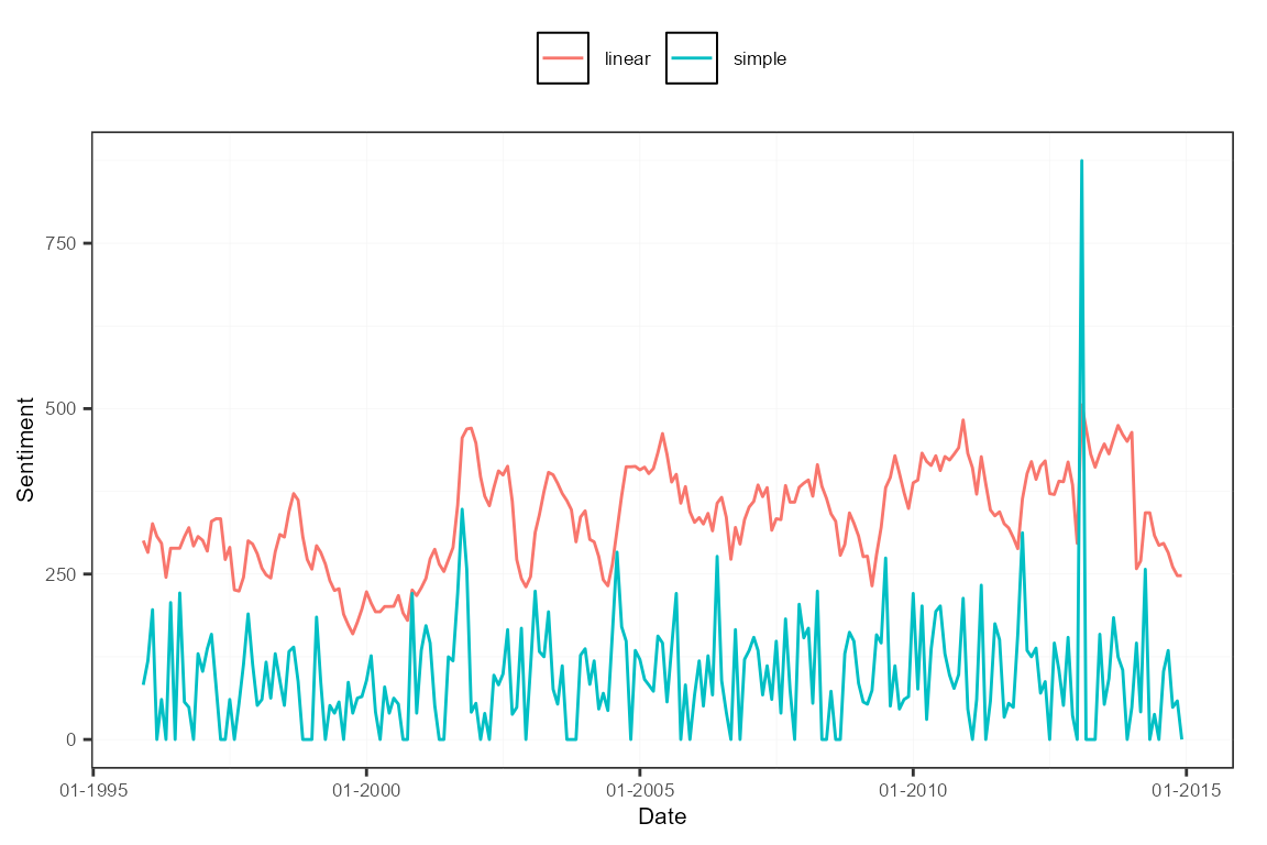
This new sentiment object is aggregated into a monthly
average and a 12-monthly linear moving average time series per
newspaper. Setting howDocs = "equal_weight" and
do.ignoreZeros = FALSE normalizes the monthly values by the
combined number of news articles in that month.
w <- data.frame("simple" = c(rep(0, 11), 1), "linear" = weights_exponential(12, alphas = 10^-10)[, 1])
ctr <- ctr_agg(howDocs = "equal_weight", do.ignoreZeros = FALSE,
               howTime = "own", by = "month", lag = 12, weights = w)

sm <- aggregate(s2, ctr)
Scale newspaper-level EPU measures
The next step is to scale the newspaper-level EPU time series to unit standard deviation before a certain date (in this case, before 2005). Rather than unit standard deviation, we standardize to a standard deviation of 100.
dt <- as.data.table(subset(sm, date < "2005-01-01"))
sds <- apply(dt[, -1], 2, sd)

sm2 <- scale(sm, center = FALSE, scale = sds/100)
subset(sm2, date < "2005-01-01")[["stats"]]
## EPU--wsj--simple EPU--wapo--simple EPU--wsj--linear EPU--wapo--linear
## mean 96.1926353 76.9955241 319.1703100 271.85568619
## sd 100.0000000 100.0000000 100.0000000 100.00000000
## max 380.3967953 389.0856498 644.9521817 526.74844061
## min 0.0000000 0.0000000 179.4097421 93.69645949
## meanCorr 0.1047356 0.1347121 0.1217423 0.08630789Aggregate measures into one EPU index
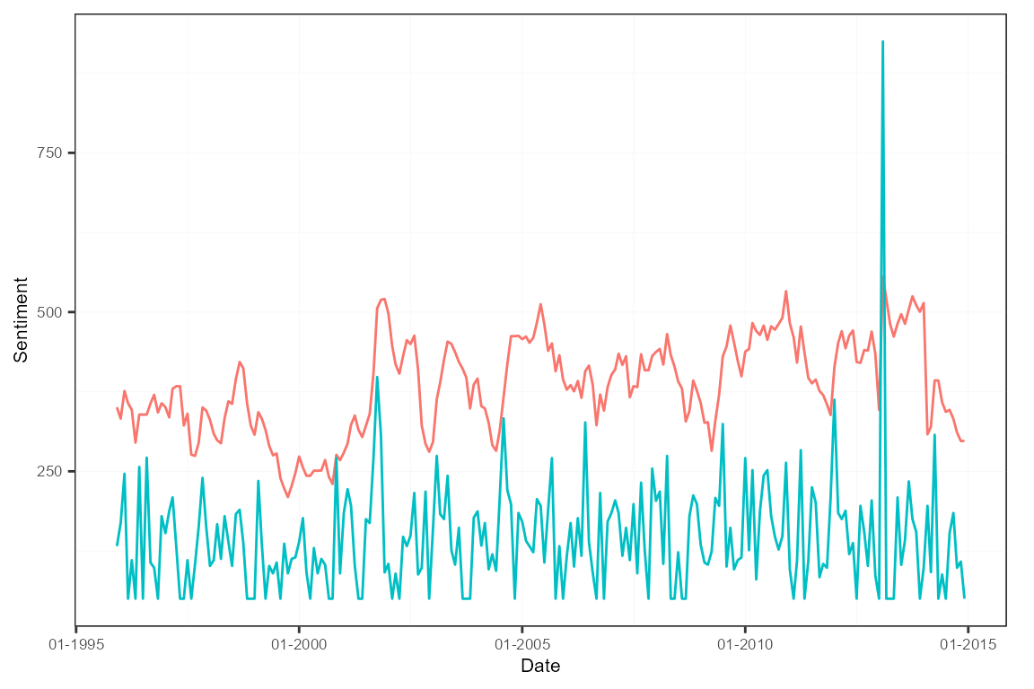
To then obtain the actual EPU index, the newspaper-level series are
averaged by reapplying the aggregate() function. We are
left with two series, one a moving average of the other.
A sentiment-adjusted EPU index
A sentiment-adjusted EPU index adds a layer of news sentiment analysis to the typical creation process. The resulting index will fluctuate between negative and positive values depending on how news writes about topics related to economic policy uncertainty, rather than only analyzing if they write about it.
Recreate corpus object
We start from scratch by reinitializing the corpus.
corpus <- sento_corpus(usnews[, c("id", "date", "texts", "wsj", "wapo")])Compute EPU relevance
We move forward by adding binary features to the corpus for the E, P
and U keywords defined earlier. Next, we compute an EPU feature, based
on the same mechanism using the self-created to_epu()
function.
corpus <- add_features(corpus, keywords = keywords, do.binary = TRUE)

dv <- as.data.table(docvars(corpus))
dv[, EPU := to_epu(.SD), .SDcols = c("E", "P", "U")]
Add normalized newspaper features
Having detected the news articles to count in the EPU index, we need
to normalize these counts. We do so per newspaper using some
data.table magic, and then add the
appropriate features to the corpus using
add_features().
# compute total number of articles per journal and month
totArticles <- dv[, date := format(date, "%Y-%m")][,
  lapply(.SD, sum), by = date, .SDcols = c("wsj", "wapo")]
setnames(totArticles, c("wsj", "wapo"), c("wsjT", "wapoT"))

dv <- merge(dv, totArticles, by = "date")
dv[, c("wsj", "wapo") := list((wsj * EPU) / wsjT, (EPU * wapo) / wapoT)]

for (j in which(colnames(dv) %in% c("wsj", "wapo"))) # replace NaN and Inf values due to zero division
  set(dv, which(is.na(dv[[j]]) | is.infinite(dv[[j]])), j, 0)

corpus <- add_features(corpus, featuresdf = dv[, c("wsj", "wapo", "EPU")])
Select EPU corpus
We continue with a subsetted corpus carrying those articles discussing enough EPU material. We clean the features keeping only the normalized newspaper-level features.
corpus <- corpus_subset(corpus, EPU == 1)
docvars(corpus, c("E", "P", "U", "EPU")) <- NULL
Aggregate into a sentiment-adjusted EPU index
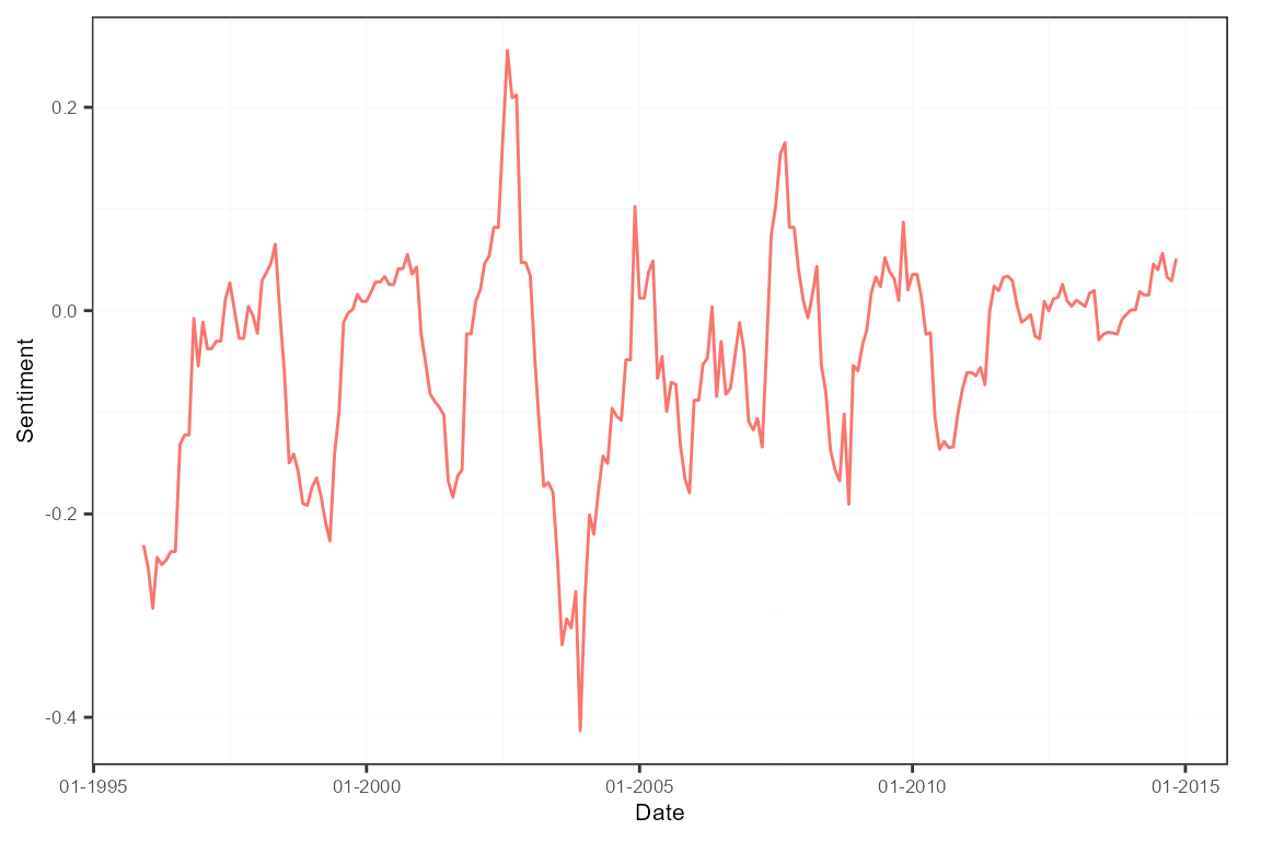
The news sentiment layer is added by applying the all-at-once
sentiment computation and aggregation function
sento_measures(). The popular Harvard General Inquirer is
the sentiment lexicon at service. Averaging across the newspaper series
gives a final EPU index. Specific scaling as shown before is left
aside.
sentLex <- sento_lexicons(sentometrics::list_lexicons[c("GI_en")])
ctr <- ctr_agg("counts", "equal_weight", "equal_weight", by = "month", lag = 12)

sm <- sento_measures(corpus, sentLex, ctr)

sm2 <- aggregate(sm, features = list(journals = c("wsj", "wapo")))

plot(sm2)